Evolutionary algorithm assisted antenna design
Before I began I needed to learn a bit about VSWR. VSWR stands for Voltage Standing Wave Ratio. It is a measure of how much power is being reflected back to the source from the load. It typically written as a ratio like 2:1 or ∞:1 or as just the first number in that ratio (ie. 2:1 ⇛ 2). In a perfect scenario the VSWR would be 1 where 0% of the power is reflected back to the source and is all used by the load. The worst scenario is where 100% of the power is reflected back and this is the VSWR of a short-circuit. In essence, the VSWR of an antenna is the amount of power radiated by that antenna, lower is better.
The requirement for the final design was that the VSWR has to be less than or equal to 2.5 for the frequencies of 108MHz to 162MHz and 225MHz to 400MHz, but that essentially means that the antenna has to work for the whole range of 108-400. If a suitable antenna shape couldn't be found then a tuned antenna would be used which uses electronics to modify the antennas shape to better perform at the chosen frequency. Tuned antennas are vastly more expensive and complex.
The antenna must fit in roughly 27cm tall and 75cm wide space. This makes low-frequency antenna design difficult because the wavelength for the lowest frequencies is 2.7m (2.6m in conductors) which is much larger than the available space.
The first few challenges of this project are about representation and fitness. First is to decide what makes a good antenna, since the specification is clear that the VSWR needs to be below a certain value over a certain range I defined fitness as the average VSWR over the range 108-400MHz. Second, I must decide on a representation for the antenna, this representation matters a lot because it will determine what “similar” antennas are from an evolutionary perspective, ie. two antennas where one mutation can make either one. Ideally, similar antennas from an evolutionary perspective have similar characteristics, namely fitness. I decided the representation would likely be a matrix but left the specifics until later.
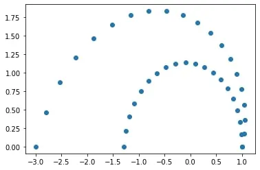
After researching existing antennas, I figured that I would try to recreate some of them and see if I could get similar results using the windows version of 4nec2, the Python version necpp and a real world sheet of metal. The chosen antenna design was a scimitar antenna like was used in the Apollo program. I wanted to get a list of points on the path of the scimitar that I could later feed into necpp. Using the patent I parameterized the two curves (k e^(at) cos t, k e^(at) sin t) and wrote some code to generate and plot the points. Which for a specified number of segments returned this:
Next, I wanted to test that antenna in necpp, to do that I first needed to familiarize myself with the necpp library. I found some example code from the PyPi Website. It simulates a vertical pole and calculates the impedance for the frequency 34.5 MHz.
def handle_nec(result):
    if (result != 0):
        print (necpp.nec_error_message())

def impedance(frequency, z0, height):
    nec = necpp.nec_create()
    handle_nec(necpp.nec_wire(nec, 1, 17, 0, 0, z0, 0, 0, z0+height, 0.1, 1, 1))
    handle_nec(necpp.nec_geometry_complete(nec, 0))
    handle_nec(necpp.nec_gn_card(nec, 1, 0, 0, 0, 0, 0, 0, 0))
    (necpp.nec_fr_card(nec, 0, 1, frequency, 0))
    handle_nec(necpp.nec_ex_card(nec, 0, 0, 1, 0, 1.0, 0, 0, 0, 0, 0))
    handle_nec(necpp.nec_rp_card(nec, 0, 90, 1, 0,5,0,0, 0, 90, 1, 0, 0, 0))
    result_index = 0

    z = complex(necpp.nec_impedance_real(nec,result_index),
            necpp.nec_impedance_imag(nec,result_index))

    necpp.nec_delete(nec)
    return z

z = impedance(frequency = 34.5, z0 = 0.5, height = 4.0)
print ("Impedance \t(%6.1f,%+6.1fI) Ohms" % (z.real, z.imag))
The library works with cards, a holdover from actual punch cards, that are used to define aspects about the simulation. For example, the nec_fr_card allows me to change some frequency information about the simulation. After getting that to work, I tried simulating multiple connected wires, with the goal of eventually putting together a scimitar geometry. When I ran that though, I got an error, "index 2 is out of bounds for axis 0 with size 2" or sometimes just a crash. The lack of good documentation and examples made debugging difficult, but eventually I figured out the problem was with the segment count. I brute forced my way to a segment count that worked for the shape I was trying, which would be good enough for now. Later, I found out that the segment count must be high enough so that the largest segment of a wire is smaller than 20% of the wavelength. Basically, divide the speed of light by the highest frequency, divide that by 5 and make sure the wire has enough segments so that they are all smaller than that value. From there I could calculate the impedance for a specific frequency for any geometry I wanted, the final code looked like this:
def impedance(freq,pts):
    nec = necpp.nec_create()
    for a in range(0,pts.shape[0]-1):
    y1=pts.item((a,0))
    z1=pts.item((a,1))
    y2=pts.item((a+1,0))
    z2=pts.item((a+1,1))
    handle_nec(necpp.nec_wire(nec, a+1, segmentCount(y1,z1,y2,z2), 0, y1, z1, 0, y2, z2, 0.001, 1, 1))

    handle_nec(necpp.nec_geometry_complete(nec, 1))
    handle_nec(necpp.nec_gn_card(nec, 1, 0, 0, 0, 0, 0, 0, 0))
    handle_nec(necpp.nec_fr_card(nec, 0, 1, freq, 0))
    handle_nec(necpp.nec_ex_card(nec, 0, 1, 1, 0, 1.0, 0, 0, 0, 0, 0))
    handle_nec(necpp.nec_ld_card(nec, 5, 1, 0, 0, 58001000, 0, 0))
    handle_nec(necpp.nec_xq_card(nec, 0))
    result_index = 0
    z = complex(necpp.nec_impedance_real(nec,result_index),
            necpp.nec_impedance_imag(nec,result_index))


    necpp.nec_delete(nec)
    return z
Which returns the real and imaginary components of impedance for a certain frequency (freq) for a given list of points (pts). Impedance could then be turned into VSWR using an equation found here. To properly evaluate an antenna, I need a way to find the VSWR for multiple frequencies. Originally, I called the impedance functions for every frequency in the range, but this was needlessly slow because the program had to rebuild the geometry and environment each time it tested a frequency. By changing the frequency card (fr_card) I could calculate the impedance of multiple frequencies and then return them as a list.
Finally, I could test out the scimitar. To get better results, I moved the tip of the scimitar to (0,0) and the wide part of the scimitar off the ground plane. To fit in the available space, I scaled the scimitar of the patent slightly. Here is the antenna I tested:
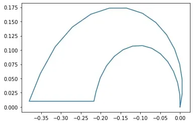
And the resulting VSWR graph:
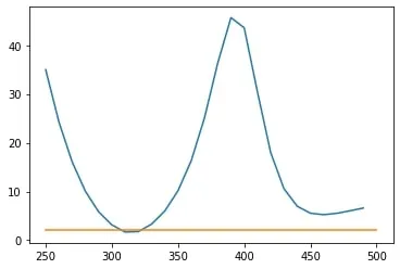
The scale is in meters and orange line marks a VSWR of 2.5, which is the goal for the whole frequency range.
Clearly, the antenna as-is was not good enough for the job, but it was possible with the right set of parameters it could work. Before subjecting it to an evolutionary algorithm, I had to choose some parameters that would determine the specifics of an individual scimitar antenna. The 4 that I chose were a horizontal scaling coefficient, inner and outer curve values, and scale. I set boundary conditions for the antenna so that they would be a reasonable size (not good ones though because the output antenna ended up being about a meter long). Next, I modified the existing code to test the scimitar geometry and output its score as a sum of all the VSWRs in the chosen range to optimize, this was the cost of an organism.
Then I just had to implement the evolutionary algorithm. The core steps in an evolutionary algorithm are evaluation, selection, and variation. A random sample is generated and then these three steps are iterated as many times as necessary. Evaluation is the process of determining the most fit individuals (or least costly). Selection is the process of destroying the least fit individuals. And finally, while there are many different possible implementations of variation, the basic goal is to replace the lost population with combinations of the successful organisms with some random variation. As an example of variation, if an organism is represented by a binary number, the first half of one and the second half of another successful organism could be combined. Mutation could be implemented by flipping some number of bits in the new organism. I took the best half of organisms according to the cost and averaged random individuals to create the new population, additionally I added or subtracted small numbers to act as mutation. After running it for 500 generations with a population of 500 the result looked like this:
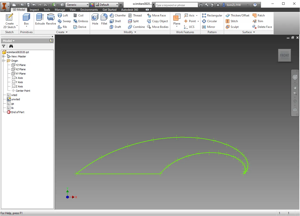
which gave a VSWR graph that looked like this:
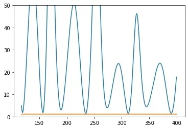
where the y-axis is 0-50 and the x-axis is 118 to 400MHz. After that I tried a few other optimization strategies. First, putting a 3 times weight on all frequencies higher than 250MHz which yielded this antenna:
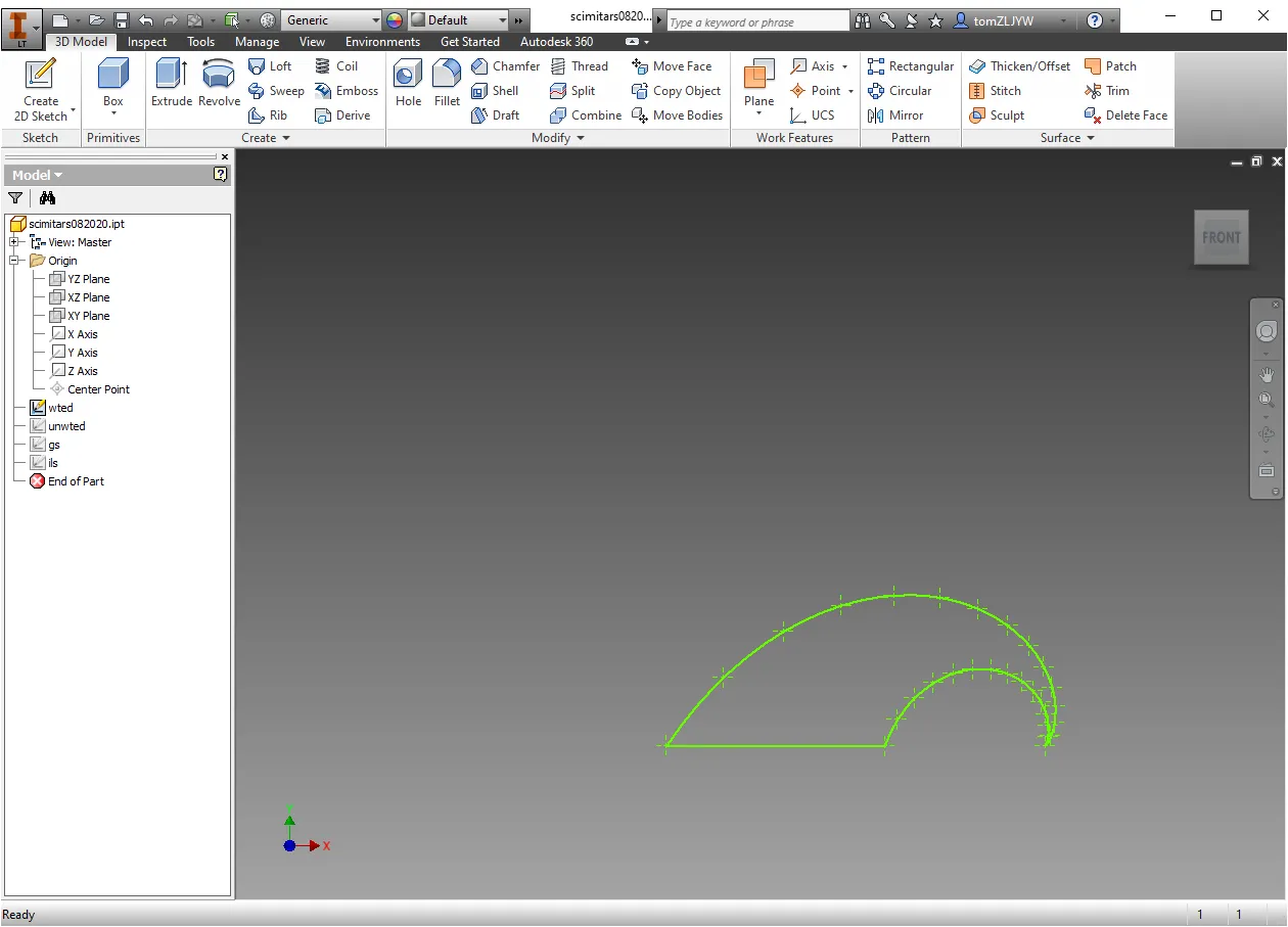
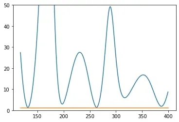
Which gave this VSWR graph (same axis):
I wanted to see if real versions of the antenna would give similar VSWR plots as the simulated ones. After drawing out the scimitar shapes on some paper, gluing tinfoil to that paper and cutting out the shapes, I tested the geometries. It turns out tinfoil gives the same VSWR values as a metal plate of the same shape, antennas are just made out of .032" aluminum so they don't melt. Outlines of wire also (supposedly) give the same VSWR as a filled in sheet which should mean that nec correctly simulates plate antennas. The actual sweep of the second antenna looked like this:
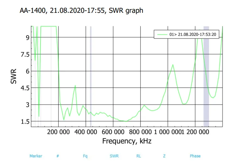
With x-axis from 0-1400MHz. The shape is similar in the range 118-400 but the values are considerably lower in the real world. This is probably fine because if the shape of the graph is similar then an optimized version will still be optimized in the real world and just have a better VSWR.
The scimitar seemed unlikely to work well enough to meet the requirements for a few reasons. First, all the antennas were too big but still gave VSWRs not close to the goal. Also, scimitars are usually used for narrow high frequency ranges and are seemingly can’t work well in lower ranges as I'd hoped. While there are a few options for existing designs to optimize (a U like design, multiple vertical wires, scimitar variants and trapezoidal shapes) I really wanted to see if a generalized antenna evolver would work.
I started by defining a rectangle that bounded where points could be, about 25cm tall and 60cm wide and defined a shape that would be on every antenna a 2cm by 1cm triangle where the antenna would be attached (with an alligator clip for testing but eventually soldered). Then, I defined an individual as a collection of points (a 2 by N matrix to represent the x and y position of N points) in the order that they would be connected by wires which would outline a shape. For example, an individual with a matrix of points like this:
[[ 0.          0.        ]
 [ 0.01        0.01      ]
 [ 0.1056655   0.2056655 ]
 [ 0.262       0.32031084]
 [ 0.262       0.4673137 ]
 [ 0.262       0.60390589]
 [ -.1347361   0.70804492]
 [-0.01        0.01      ]
 [ 0.          0.        ]]
Which gave this outline:
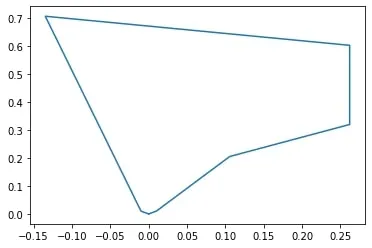
Notice the small triangle at the bottom of the antenna, that's the preset shape that allows the antenna to be attached, every matrix has the points (0,0) and (0.01 , 0.01) at the beginning and a similar set of points at the end to define that shape. All I had to do was make some small modifications so that the testing code would take in the new representation. There's one big problem, my code can’t really handle geometry errors. If two wires cross, it breaks, if two wires are too close together, it breaks, and if the wires are in certain configurations, it returns negative VSWRs (it breaks). Luckily, all the necpp functions return an int, 0 if it ran without errors, and some other number if there was an error (different numbers for different errors). I can find negative VSWRs because the real component of the impedance is negative. I use that result to check if there are any errors when calling a function and if there are, I give the broken antenna a high VSWR which should make it worse than any working antenna. I didn't have to do this for the scimitars because I set the limits on the individuals such that they would all give working shapes.
After running this new implementation in Google Colab, the program would eventually crash, without error. I figured that the problem was that I was running out of memory but after running it a few more times that didn’t seem to be the problem. Since memory didn’t seem to be the problem, I guessed that some antenna configuration might cause necpp to get caught in an infinite loop or crash. To see if that was the case, I added some print statements to print out all the “individuals” in a generation, unsurprisingly, this made the program too slow, and it never encountered the problem. While Google Colab had been great for a few reasons, it supported necpp and was faster than my laptop, it seemed that I would have to leave it behind. After downloading Oracle VM and installing Ubuntu, necpp is Linux only, I copied over my code, replaced print statements with writing the to a text file, and ran the program. After a few hours, the program stopped, just like it had in Colab.
To see if it was one of the antenna shapes that made it break, I got rid of the code that made random individuals at the start and replaced it with code that read in the saved generation from the text file. It ran fine. So, it wasn’t the specific antenna shapes that made it break. I had no idea what else to try, after a while, the code just stops. I noticed that the more times I load in the generations after it stops, the shorter it runs for, so obviously there is some dependence on what the generation looks like, but I still don’t know why the code is broken.
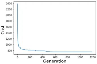
Luckily, in testing that theory, I had also built a workaround. I could just run the code until it stopped, exit the program, and restart the program loading in the saved generation. If I did that a few times then it would be as if the program had run longer. This also isn’t as much of a problem as I’d feared because individuals stop improving after a while. Here is the graph of how the best individual scores as a function of generation, I looked a few of these graphs and they all follow the same pattern.
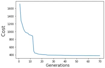
Also, some runs seem to get stuck early on with a bad design, in which case I just restart the program, the graph for those runs looks like this.
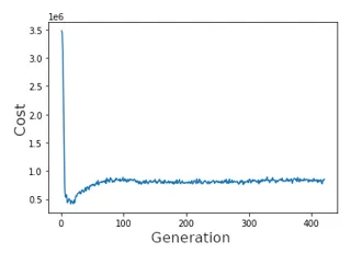
Interestingly, while the graph of the best individual’s core follows a roughly exponential decay, the average score of a generation is very differently shaped. Again, this is an example of just one run but all of them take on a very similar shape.
After running it about 6 times (with about 3 “restarts” per) I collected the best individual from each run. I then selected the two best scoring designs to test in the real world. They looked remarkably similar:
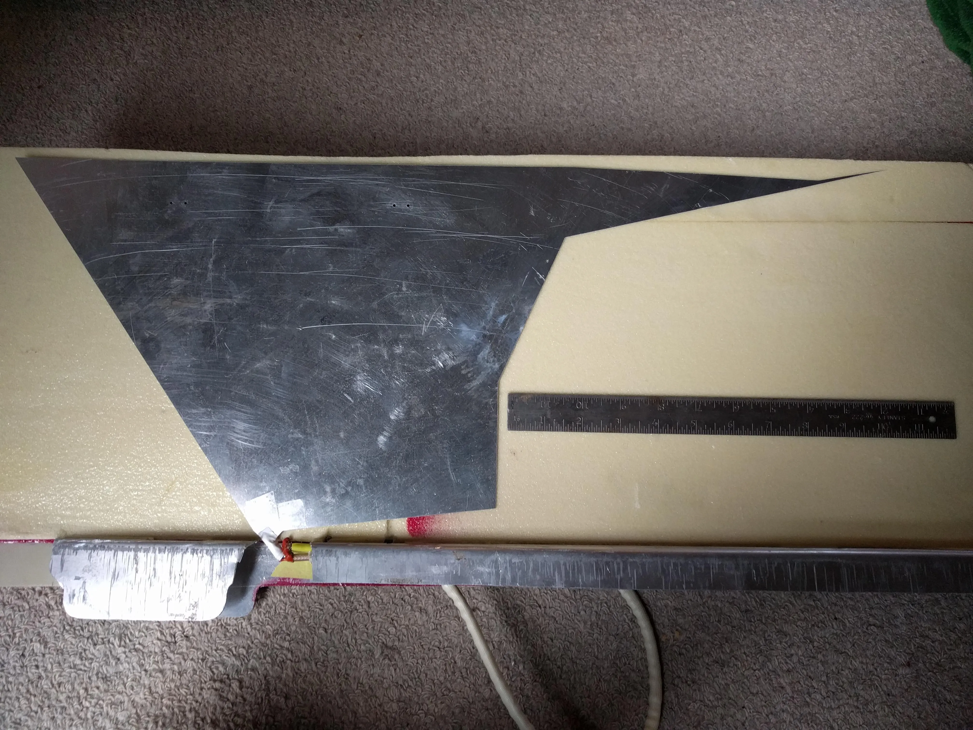
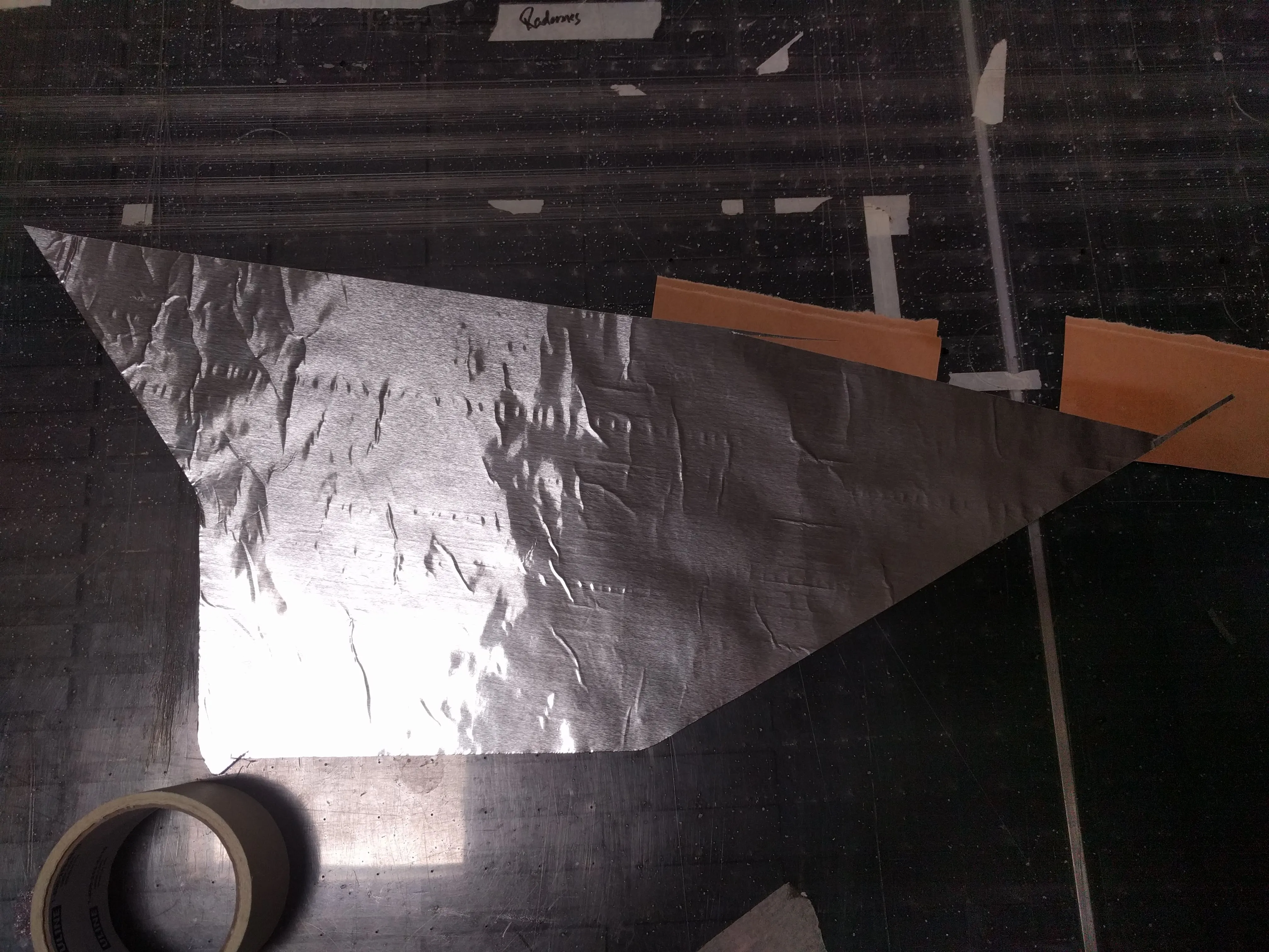
They both had a generally trapezoidal shape, took up the maximum height and had a extended part on the right top size. This seemed good, if the algorithm had converged on similar shapes over multiple independent executions, that would suggest it was optimal in some way.
I cut them out using the same technique I had used to test the scimitars, thick paper glued to tinfoil cut out with a CNC-like cutting machine. Then I taped them to the test stand, attached them with an alligator clip and put them on the tail, the testing setup looked like this:
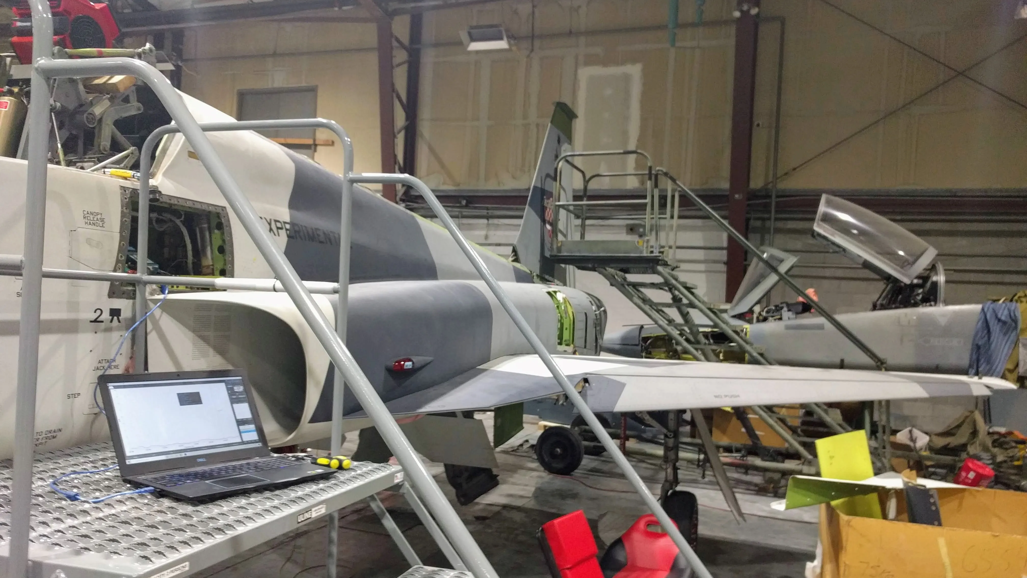
I tested the first antenna, giving the following VSWR scan, the red and green lines are two trials, with essentially identical results.
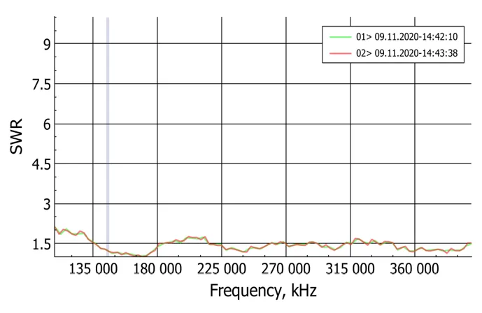
For reference this is the VSWR scan on the old design, the highlighted section is the same range as the previous image.
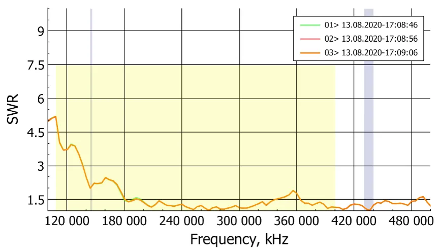
Way better, and even more important, better than spec. The other design was alright, but not as good.
In the end, the final design was cut out of aluminum and tested again, just to make sure, with
identical results. That antenna was then shipped off to a third party who verified the results and
additionally did some analysis on the directionality of the signal, which showed that the new design
was no more directional than the old design. This project shows the significant potential of
evolutionary design, with relatively little domain knowledge I was able to design a fixed antenna
that outperformed the old design and exceeded specification. Afterwards, I wrote a paper, Evolutionary Algorithm Designed Broadband Plate
Antenna for F-5 Vertical Stabilizer, that goes through the requirements, methods, and
results in additional detail.
A* Pathfinding
The objective of a pathfinding algorithm is to find the shortest path between two points. For this particular project, the path was on an NxM grid where some grid points are marked as obstacles. I first implemented Dijkstra’s shortest path algorithm which would be extremely slow for the given use case but was simple to implement and helped me understand the core algorithm behind A*. With Dijkstra’s complete I moved on to more advanced algorithms that take advantage of extra information, A*, for example, uses the fact that an approximate distance can be found between two points which lets the algorithm search more effectively.
With a better understanding of the algorithm, I moved on to implementing A*. Deciding that now was as good a time as any, I also created some test cases using JUnit. After all, if it’s not tested, it's broken, and wouldn’t you know, it was broken. After some significant debugging, I realized my mistake, as an optimization, I had only created an instance of the point class when I “discovered” a point, what I had done wrong was to instantiate a new point even if it had already been discovered. Honestly, with such a major oversight I was shocked at how few test cases it failed. To fix this I used Java’s HashMap to store all the discovered points and only created one if it didn’t exist.
After testing with JUnit and benchmarking A* I was surprised at how slow it was. Looking for ways to speed it up I found an algorithm that takes advantage of the regularity of the grid called jump point search (JPS), which is said to be significantly faster. The original idea for JPS comes from this paper by Daniel Harabor and Alban Grastien and I found this website by Nathan Witmer to give a great visual intuition behind the algorithm. Unfortunately, for almost every obstacle placement I found JPS to be slower than traditional A* and for very large grids it would run into the recursion limit.
Still looking for a faster implementation, I tried to optimize by original A* implementation. I did so first by writing my own priority queue implementation that supported an ‘increase priority’ method, and second by condensing the representation of a grid point. Originally, I had a grid point class that stored the g-cost, f-cost, parent point, and x and y coordinates of the point. While this was simple and readable, it came with all the overhead of a Java class, which for many points added up. I was able to reduce all the information down so that it was able to fit into a single long (a 64-bit number), then I built a class to abstract that structure away from the core A* algorithm. This helped quite a bit but was still slower than I would have liked.
I decided to code the algorithm in C. It would be a good opportunity to refresh some basic C and should yield a faster implementation. I decided that I would start by implementing a linked list which I used to store the final path. I also decided to use the linked list for my priority queue implementation, just iterating over the whole list and then returning and splicing out the “minimum” element. I knew this would be very slow (O(n) as opposed to O(lg n) using a binary heap) but it would let me debug the A* algorithm, give me some extra practice in C and give me an idea as to the speed of C compared to Java. Additionally, instead of using a hash map to store the discovered points I just used an array with all of the potential points, while this would be very memory inefficient it would be very fast and easily implemented.
After getting that implementation working, I noticed that it was actually significantly slower than Java, originally, I just attributed that to the slow priority queue, but even after I modified the Java priority queue to loop over every element (so that the two should be equivalent), C was still slower. I looked for ways to speed up the C code and made a few optimizations. First, I removed some unnecessary malloc calls, second, I used additional space to store some values that I had previously been recalculating, most importantly, I used O flags, O2 sped up the code by almost 4x.
Finally, with some guarantee that it would be faster than Java, I implemented the priority queue as a binary heap. In the end, while it took significantly more time to code than Java it ended up being substantially faster. I was able to get the code to run anywhere from 4-100x faster than the best Java implementation. Here are all of the benchmarks for each implementation (excluding Dijkstra’s because it is way too slow) the time is the average of 5 runs excluding the extremes, the unit varies by row.
| Grid Size Start → End | Grid Type | A* Java | JPS Java | A* Bits Java | A* in C |
|---|---|---|---|---|---|
| 100 x 100 (0,0) → (99,99) | empty | 11ms | 12ms | 8ms | <1ms |
| w/ open box from 2 to 66 | 51ms | 97ms | 34ms | <1ms | |
| w/ wall from (97,99) to (97,1) | 121ms | 106ms | 87ms | <1ms | |
| 1,000 x 1,000 (0,0) → (999,999) | empty | 77ms | 42ms | 23ms | 20ms |
| w/ open box from 2 to 666 | 5.1s | 9.4s | 1.5s | .24ms | |
| w/ wall from (997,999) to (997,1) | 15s | 2.1s | 2.8s | .7s | |
| 2,000 x 2,000 (0,0) → (1999,1999) | empty | 138ms | 62ms | 40ms | 23ms |
| w/ open box from 2 to 1666 | 72s | 140s | 8.8s | 2.1s | |
| w/ wall from (1997,1999) to (1997,1) | 155s | 17s | 10s | 2.86s |
Procedural Timelapse Photos
The first method that I wanted to try was to take columns of pixels from different frames of the timelapse. This would be easy to implement and give me a rough idea of how a more advanced method would look. I would specify the width of the final image and the width of the column I'd take from each frame. From that, the final image could be constructed. The result is bands of pixels from separate frames arranged next to each other.
Before testing it, I had to find some timelapse footage, I considered taking it myself, but I needed something easy for a proof of concept, so I looked to YouTube. It's surprisingly tricky to find 24h time-lapses of interesting things with still cameras on YouTube (most are of the night skies, which stay relatively similar throughout the video, have moving cameras, have watermarks, or are of boring subjects.) I found two that work well enough for experimentation but suffer from one of the above issues: 30 Days Timelapse at Sea | 4K | Through Thunderstorms, Torrential Rain & Busy Traffic by JeffHK, and 24 Hour Time Lapse by Bob Clark. The first has a watermark and text plus I found out everything happens too fast for this method to work effectively, the second is just a boring subject and the total number of frames is a bit too short to do everything I wanted (925 frames) but was great for testing because there's a good span in time but not much changes frame to frame. The last video I found was Timelapse Los Angeles / Santa Monica Beach California by Mark From Denmark. This was a good video with a still camera and an interesting subject over a long enough time that there was good variation but unfortunately, the video is super short. There are only 616 frames and only 470 of those are useful (the rest are black or darkened from a fade in and fade out).
To get the frames of the I downloaded the YouTube videos using one of many online tools, they're kind of sketchy if you're careful to only download the video they seem to be fine, then I used VLC Media Player to get frames. Later, I would streamline this process using the library youtube-dl to download videos and FFmpeg to get all the frames as .jpg images.
I then used PIL to get pixel data from each frame. My final code simply creates a black image of the appropriate width and height and then fills it in with pixels in some nested loops, the final image is then shown. The result of the first attempt is a little underwhelming but shows some promise and some areas for improvement. Here it is on the 30 Days at Sea and the 24 Hour videos.
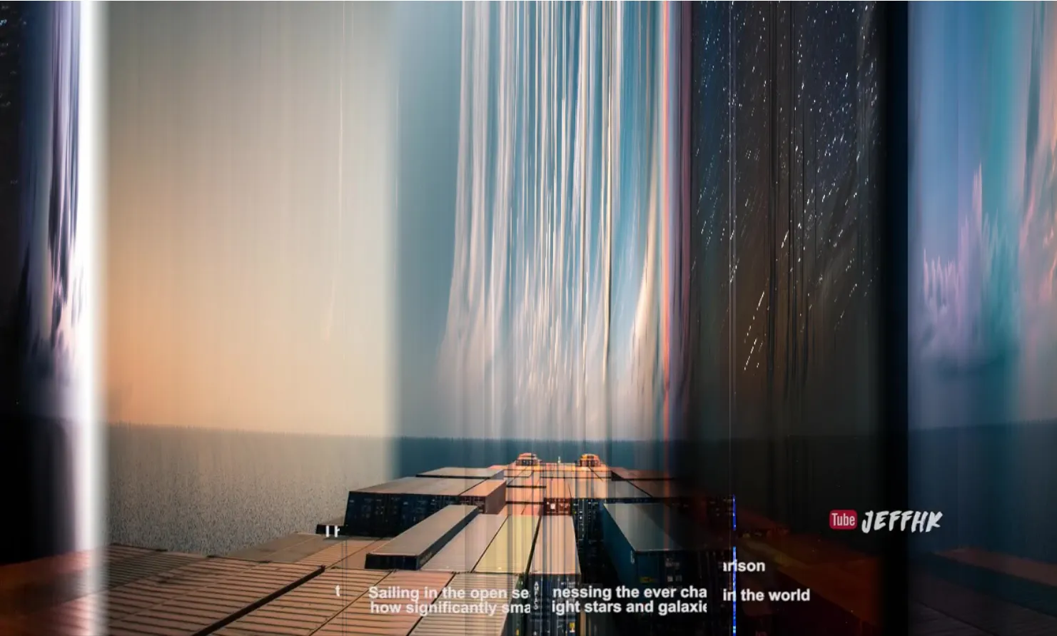
This has one pixel (column) per frame and a width of 1200 pixels.
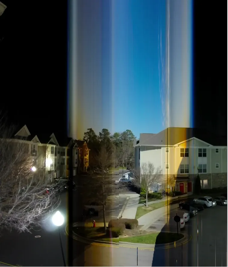
This one is 925 pixels wide and 2 pixels per frame.
There are a few issues to this method, first, the width has to be manually capped by the number of pixels per frame and the length of the video second, it just doesn't look that great, if more than 1 or 2 pixels are used in each band, they become extremely obvious. Below is an example with 4 pixels per frame and you can see clear bands start to appear.

While I think this is a good proof of concept that can make interesting images, it's not a great method.
For my second iteration, I would generalize the process by taking pixels from different frames based on a more arbitrary function. For example, the distance of a pixel from the center would decide what frame that pixel would be taken from. This solved the issue of manually setting the width and number of pixels per column, the final image would have the same dimensions as a frame from the video and the pixel distribution would be decided by the function. I ended up having a scaling coefficient to the function determined by the maximum value of the function and the size of the “useful frames” of the video. There’s still some manual parameter tuning. but I suppose this whole project is more art than science anyway. Doing this for every pixel should create a picture that would smoothly blend over the length of the video.
After implementing this more general form, the time to build an image skyrocketed from just a few seconds to an hour at which point I ended the program. What was taking so long? It turns out that while my first implementation only opened each image once (400-1,000 images), the new one opened a new image for every single pixel, about 2 million. This was obviously a complete waste of time. Fixing it required splitting the process into two steps, first, assign every pixel a frame based on the distance function and store that information in an array, second, open each image once and copy the pixels from that frame to the final image. This sped it up immensely and the code was back to running under a minute. Eventually, I decided it would be easiest to get all the pixel data from every frame, store that in a NumPy array, and then simply grab the data when I needed it. I folded this array-building process into some separate code that included the video download and frame extraction. After running this code with the center distance function on the Santa Monica Beach video I got this image.

Much more interesting. However, after finishing that implementation, I noticed that the resulting pictures had noticeably rough transitions between pixels.

To fix this, I decided to use a weighted average of a pixel’s value over some time, this should soften the transition essentially by “blurring” the photo over the time axis. I was hoping this would mimic the effect of long-exposure photography. This new method took significantly more computer power, while the original version sampled just 1 value per pixel the new version would sample 64 pixels and then perform a weighted average, which took additional time.
To speed up the new version I looked to parallelize the computation using the multiprocessing library. I further optimized the code by precomputing the Gaussian distribution (which is what I used as the weighted average values), pre-retrieving the image pixel values and storing them in an np array, and doing all three color channels at once using a matrix multiplication rather than doing the dot-product on a per channel basis, after that I was able to get the time to build an image down to around 10 minutes on my laptop, still slower than I’d like but not excruciatingly slow.

There are still some noticeable artifacts that I suspect come from YouTube's video compression being compounded by averaging over many frames, especially around the ferris wheel. Additionally, with this new technique, some of the color detail and contrast is lost in the ferris wheel which is something I might revisit. I'd like to take some of my own timelapse videos and use this tool and see what results I can get.